This article explains how the Adaptive On-Line Page Importance Computation (AOPIC) algorithm works. AOPIC is useful for performing efficient broad crawls of large slices of the internet. The key idea behind the algorithm is that pages are crawled based on a continuously improving estimate of page importance. This effectively allows the user of the algorithm to allocate the bulk of their limited bandwidth on the most important pages that their crawler encounters.

Similarly to the famous PageRank algorithm, AOPIC iteratively determines page importance based on the degree to which other pages link to it. What’s particularly nice about AOPIC is that it is simple to understand and implement, uses little memory and computational resources, and allows the user to control how much discovery of new pages should be favored over making a more accurate importance estimate.

Getting a sense of page importance and prioritizing the exploration of more important pages is critical in real-world use-cases of broad crawls. For example, in order to make the best use of their network, an internet archiving service like Internet Archive’s Wayback Machine or Common Crawl has to decide which sites are important to update frequently, and which can be visited only occasionally. As another example, an advertising agency might wish to get a sense of which topics different publishers tend to write about, and what the general quality of a publisher’s content is in order to more effectively allocate their ad inventory. Since pages are constantly added and removed from the web and can change over time, they have to continuously update and refine their importance estimates with something like AOPIC.

This article starts by introducing a simplified version of AOPIC that works on a finite, unchanging graph–a simple mathematical abstraction of a network like the internet. This will allow us to actually run a version of the algorithm in the browser. Next, we explain how to overcome the limitations of this approach by generalizing the simple algorithm to work well on a dynamic, virtually infinite graph like the real internet.

The code that runs the AOPIC widgets that appear later on in this article is available from our intoli-article-materials repository. Feel free to use it as a starting point for your own projects, and consider starring the repo! It’s a great way to find out about upcoming articles before they’re released, and to send us a signal about the kind of content you would like to see more of.

OPIC: A Basic Version of the Algorithm

The internet can be mathematically abstracted as a directed graph. Each page becomes a node in the graph, and each link becomes an arrow between the nodes.

In this article, instead of labeling nodes with the urls they correspond to, we’ll use integer labels or simply leave them unlabeled. Under this representation, the actual internet would be a graph with infinitely many nodes due to the presence of dynamically generated pages. For example, a lot of sites employ infinite link cycles or “bot traps,” while others use JavaScript to render some meaningful content on every path under the domain. Even ignoring these pages, we’d end up with a graph so large so as to be virtually infinite for all practical purposes. Moreover, the internet’s graph changes from moment to moment, so any graph representation would immediately become outdated.

In order to get the basic concepts of the algorithm down, we’ll start with a version which operates on a finite, unchanging graph with $n$ nodes, each corresponding to a page. Later, we’ll cover the extension of the algorithm to more realistic, arbitrarily large graphs. To simplify things further, assume for the moment that every page has at least one link to another node. This assumption hints at a technical requirement for the algorithm to work, and we’ll cover this in some more detail a little bit later. Since this version of the algorithm doesn’t account for a changing graph, the authors of the AOPIC paper dropped the first word, “Adaptive,” from the name, naming it On-Line Page Importance Computation (OPIC).

The OPIC algorithm uses a credit system to calculate the importance of every node. A finite number of credits, 100 say, are allocated to the nodes of the graph, and then swapped around as nodes are “crawled.” Each node $i$ has two numbers associated with it: the total number of credits currently allocated to the node, called the “cash” $C(i)$ of the node, and the sum total of credits that were previously associated to the page, called the credit “history” $H(i)$ of the node. With these definitions out of the way, we can describe how the OPIC crawling algorithm works:

1. Initialize each node by allocating the same number of the total credits to it, and setting its history to 0. If there are $n$ nodes in the graph, then we are just initializing the graph with $C(i) = 100/n$ and $H(i) = 0$ for all $i$.

2. Choose a node $i$ using some crawling policy, such as random selection.

3. Add an equal portion of $C(i)$ to every node which node $i$ links to. If node $i$ has $m$ edges to other nodes, then we would add $C(i)/m$ to each of them.

4. Increment the node’s history $H(i)$ by $C(i)$ and set $C(i) = 0$.

The idea is that over time you allocate more credits to the nodes that are linked to the most. If the edges come from other nodes which themselves have a lot of inbound edges, then these will naturally receive more credits than nodes which are linked to from nodes with few inbound edges. Each node’s importance is at any given time defined as the total portion of credits in the system that have been assigned to the node so far, and it’s clear that this importance estimate improves as we crawl more nodes. Mathematically speaking, after the $t$-th iteration of the algorithm, we define the importance $X_t(i)$ of node $i$ “at time $t$” as

$$ X_t(i) = \frac{H(i) + C(i)}{\sum_i H(i) + 100},. $$

The cash and history of the nodes also obviously change with time $t$, but we will only keep track of their latest values and therefore avoid subscripting them.

It can be proven that as long as each node is crawled infinitely often, then $X_t(i)$ will converge to some value as the number of iterations $t$ of the algorithm goes to infinity:

$$ X(i) := \lim_{t\to\infty} X_t(i) ,. $$

It also turns out that the error of convergence at any time $t$ is inversely proportional to the total history of the system, $\left| H_t \right| = \sum_i H(i)$, which is just sum of the current history of every node in the graph at time $t$. So, we can stop the algorithm when the value

$$ \frac{1}{\left| H_t \right|} $$

stops changing by very much.

Demo of OPIC

To get a clearer sense of the cash allocation process, let’s run the algorithm on a toy graph in the browser. The following widget lets you run the algorithm to see how the values update. You can manually go forward step-by-step, or press play and see the values update over time (control the speed by pressing - for slower iterations and + for faster iterations). By default, each node is represented by a circle with two numbers in it. The top number is the node’s current cash, and the bottom number is the node’s previous credit history. You can instead show each node’s importance by toggling between them using the controls.

For now, we’ll just use random selection as the “crawling policy”, since the graph is small and will stabilize pretty quickly. We’ll get rid of that policy a little bit later.

After running the simulation for a bit, you should see that the importance starts stabilizing. The node in the middle should emerge as the one with most importance, which is hardly surprising given that it’s by far the most linked to one. A few other interesting tidbits can be observed, however. First, the node in the middle of the top row ends up with almost no importance–as expected, because it has no inbound edges! Second, although several nodes share the same number of inbound edges, their importance differs. In particular, the nodes which are pointed to the more important nodes end up being more important themselves. Obviously this is a bit of a contrived example, but it is already enough to serve as a sanity check for the algorithm.

AOPIC: Generalizing the Algorithm to Dynamic Graphs

The algorithm from the previous section contained a few simplifying assumptions:

1. each node is assumed to contain a link to some other node;
2. the crawling policy is random selection; and
3. the graph is assumed to be finite and unchanging.

Obviously these don’t hold up on the real internet, so a few modifications need to be made to the algorithm in order to make it useful in practice.

Dealing with the Graph’s Connectivity

Pages online sometimes don’t have any outgoing links, which is a problem for the current algorithm because they would end up being the last stop for cash and cause it to effectively disappear from the rest of the graph. The simple way around this issue is to add a “virtual” page which every other page links to, and which links back to every other page (or a carefully chosen subset of pages at any given time–more on that in a moment). The virtual page will therefore accumulate credits during every iteration of the algorithm, and eventually be picked and distribute credits back into the system.

A Better Crawling Policy

The second issue with the simplified algorithm above is that pages are crawled randomly. While this technically gets the algorithm to converge eventually, it will be slow to do so on a large graph. If we are truly interested in spending most of our resources on the most important parts of the web, we can instead adopt a greedy crawling policy under which we choose the page with the largest amount of cash at any given time.

In fact, if we use the greedy selection policy instead of random node selection, convergence will be achieved about two times as fast–as long as we assume that cash is accumulated by pages linearly, a claim which the authors of the AOPIC algorithm confirmed by experiment and which makes sense intuitively. This is pretty easy to see, and is an interesting tidbit from the AOPIC paper, so let’s make a small diversion.

Every time a node is visited, the convergence error bound’s denominator $\left| H_t \right|$ increases by the amount of cash allocated to the page. In a graph of $n$ nodes being crawled under the random policy, each node will on average get $100/n$ of the total $100$ credits in cash on each visit, and increase the denominator by a corresponding amount. Under the greedy crawling policy, we don’t know the average cash of a node when it’s visited, but let’s call that number $\alpha$. Since after each visit the cash resets to 0, on average each node will have $\alpha / 2$ cash on it at any time. There are $n$ nodes, so in fact $100 = n (\alpha / 2)$, and so $\alpha = 200/n$. Therefore, the convergence error bound’s denominator increases twice as fast as with the random policy. Neat!

A greedy crawling policy also enables us to make tradeoffs between new page discovery and the importance learning rate. The idea is that we can modify the virtual node’s outgoing edges to bias cash allocation toward specific parts of the graph. If we were to have the virtual node point only to previously unvisited nodes, then those nodes would receive more cash over time and be scraped more often. This would in effect encourage exploration and even more new link discovery. Conversely, if were to have the virtual page point to all other nodes, then there would be no bias toward unvisited nodes, and the scraper would spend more time on the most important parts of the graph.

The following is a slightly larger synthetic example than before, this time using a greedy policy and a virtual page. The virtual page’s node is not rendered, but every time it’s picked you will see all nodes light up. If the graph is not readable for you, just hit refresh until a favorable configuration comes out–the connectivity of the graph is the same, but the physics simulation which lays out the graph settles slightly differently each time. The graph is a 24 node scale-free network (with an additional hidden virtual node), a type of graph that the internet is often assumed to be.

Importances should stabilize pretty quickly here, and you should see that the more connected nodes toward the middle of the graph become more important than the relatively isolated pages on the outside.

A Changing Graph

So far, we have only mentioned finite and unchanging graphs. On the graph of the real internet, nodes are constantly added and removed, links between them modified, and even the most comprehensive crawl eventually becomes outdated. Moreover, pages are crawled at unpredictable intervals. To deal with this, and make AOPIC out of OPIC, the OPIC algorithm can be adapted to work on a sliding time window.

The basic idea is to form an imperfect model of page importance using data from the few most recent visits to each page. A simple way of doing this arises if we again assume that pages accumulate credits linearly, because then we can easily interpolate between cash accumulated by a node since the previous visit, and the history attained by the node so far. We effectively want to “forget” about the history before the window.

To understand this more concretely, let’s fix a time window of $T$ hours and the number of hours since the last visit, the “scraping period” $S$. The latter can change between visits, so let’s consider two cases: $T < S$ and $S < T$ (we can use either one when they’re equal).

First, $T < S$. In the following plot, we plot credits allocated to some node over time. The red line captures our assumption that credits are accumulated linearly. Visits are denoted by dots on the line.

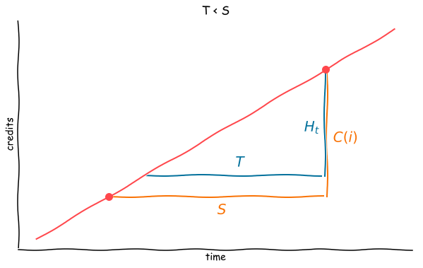
By forming ratios, we have that

$$ \frac{C(i)}{S} = \frac{H_t(i)}{T},, $$

where as before $H_t(i)$ is the history of node $i$ at time $t$, and $C(i)$ the cash accumulated since the last visit. Rearranging, we see that if $T < S$, then “resetting” the history means that we scale the cash by the fraction of credits that would have been assigned linearly to the page during the window:

$$ H_t(i) = C(i) \frac{T}{S},. $$

Next, $S < T$. This time the picture is a bit more complicated, but still just a couple of ratios stemming from similar triangles. The grey triangle indicates the period $T$ corresponding to the previous visit to the site, while the blue one indicates the period $T$ corresponding to the current period.

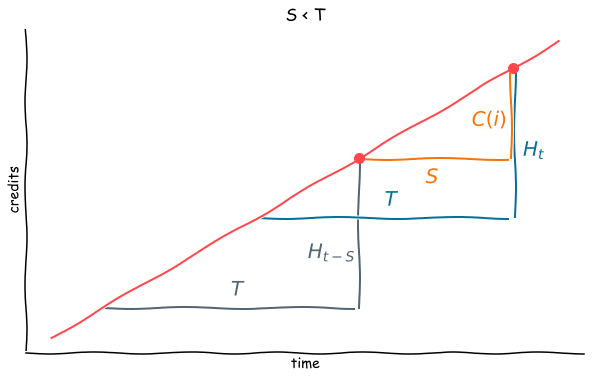
The ratios we are interested in are

$$ \frac{H_t(i) - C(i)}{T - S} = \frac{H_{t-S}}{T},. $$

Rearranging, we see that the previous history is scaled down by the portion of $T$ which falls outside the current scraping period, and then incremented by all the cash accumulated by the page during the current scraping period:

$$ H_t(i) = H_{t-S}(i) \left(\frac{T - S}{T}\right) + C(i) ,. $$

In both cases, $C(i)$ is reset to zero, and we of course have to keep track of $S$ for every page now, too.

As $T$ grows, these dynamic history estimates will approach the original definition since in that case $T - S \simeq 0$, and our importance estimates will be less and less reactive to changes over time. On the other hand, if the window size is very small, then we are for the most part just tracking cash which can cause the estimates to fluctuate. AOPIC’s authors found that a window size of 4 months is appropriate for open-ended broad crawls, but the paper was written in 2003 and the internet and web scrapers have sped up, so we can likely get good results on smaller parts on the web with substantially smaller windows. Implementing the algorithm is left as an exercise for the reader. ;)

Conclusion

If you want to dig deeper into this algorithm, there are some more details in the original paper. These include benchmarks of the convergence error bound for variations of the algorithm and its parameters, a short proof of convergence, and further comparisons with PageRank. There are also some notes about implementation, but their usefulness will depend on your specific scraping setup.

No matter how you parse the pages in your broad crawl, you will inevitably have to deal with being blocked by individual websites, as well as large networks like Distil and Incapsula. To successfully scrape large numbers of pages easily, you will need a proxy that is smart about how it routes and makes the requests. Luckily, we have just the thing for you!

If you enjoyed this article, consider subscribing to our mailing list. Another good way to follow our articles is to star our intoli-article-materials repository, since it gets updated with supporting materials for each one of our article before it’s released.