Confidence Values

If you’ve ever learned any basic statistics or probability then you’ve probably encountered the 68-95-99.7 rule at some point. This rule is simply the statement that, for a normally distributed variable, roughly 68% of values will fall within one standard deviation of the mean, 95% of values within two standard deviations, and 99.7% within three standard deviations. These confidence values are quite useful to memorize because values that are computed from data are often approximately normally distributed due to the central limit theorem. Having a rough idea of how different multiples of a standard deviation correspond to confidence intervals allows you to more intuitively understand the significance of graphs, tables, and calculations that include one standard deviation error values.

Distributions being approximately normal is certainly common, but there are many circumstances where this won’t be the case. For more heavily tailed distributions you would expect less of the distribution to fall within each multiple of the standard deviation and for less heavily tailed distributions you would expect the opposite. What if the distribution is flat or has two separated peaks? For distributions that are distinctly non-normal, those 68/95/99.7 numbers are likely to be quite inaccurate.

If you’re working with an unknown probability distribution then the confidence values for different numbers of standard deviations from the mean will also be unknown. In this situation, it becomes useful to have a “worst-case scenario” idea of how low the confidence values might be. The two standard deviation confidence value is 95% for a normal distribution, but for some distributions this confidence can be as low as 75%. That 75% value is a lower bound on the two standard deviation confidence value and it can be just as useful to keep in mind as 95% is, particularly when you’re presented with error values but no information about a distribution.

The confidence values for the normal distribution can be computed using numerical integration, but how do put limits on the confidence values for arbitrary distributions? This can be done using a bound called Chebyshev’s inequality which states that at most $\frac 1 {k^2}$ of an arbitrary distribution falls outside of $k\sigma$ from the mean. The derivation of this bound is more complicated than integrating over a distribution, but it’s relatively straightforward and should be accessible to anyone with a basic familiarity with probability and algebra. Understanding where this bound comes from, and what kind of distributions approach the bound, can be a very useful complement to the 68-95-99.7 rule in your statistical toolbox.

In this article, we’ll explore both Chebyshev’s inequality and some related concepts such as Markov’s inequality and the law of large numbers. Markov’s inequality will help us understand why Chebyshev’s inequality holds and the law of large numbers will illustrate how Chebyshev’s inequality can be useful. Hopefully, this should serve as more than just a proof of Chebyshev’s inequality and help to build intuition and understanding around why it is true.

Markov’s Inequality

Chebyshev’s inequality can be thought of as a special case of a more general inequality involving random variables called Markov’s inequality. Despite being more general, Markov’s inequality is actually a little easier to understand than Chebyshev’s and can also be used to simplify the proof of Chebyshev’s. We’ll therefore start out by exploring Markov’s inequality and later apply the intuition that we develop to Chebyshev’s.

An interesting historical note is that Markov’s inequality was actually first formulated by Chebyshev, Markov’s adviser. Chebyshev’s inequality, on the other hand, was first formulated not by Chebyshev, but by his colleague Bienaymé. Both inequalities sometimes go by other names as a result of this, but the (incorrect) attributions that we’ll use here are the ones that you’ll see most commonly.

Markov’s inequality is the statement that, given some non-negative random variable $X$ and a real number $a > 0$, the probability that $X > a$ is less than or equal to the expected value of $\frac X a$. Using $\mathbb{P}(\dots)$ to denote the probability of an event and $\mathbb{E}(\dots)$ to represent the expected outcome, we can write this inequality as $\mathbb P(X \ge a) \leq \frac{\mathbb{E}(X)}{a}$. To prove this, we begin by expressing the probability of $\mathbb P(X \ge a)$ in terms of the expectation value of a piece-wise function of $X$.

Expressing the probability in this fashion allows us to more easily make comparisons to expectation values taken over any other functions of $X$. Let’s consider the specific case of $\frac X a$ and see how this function compares to the piece-wise function.

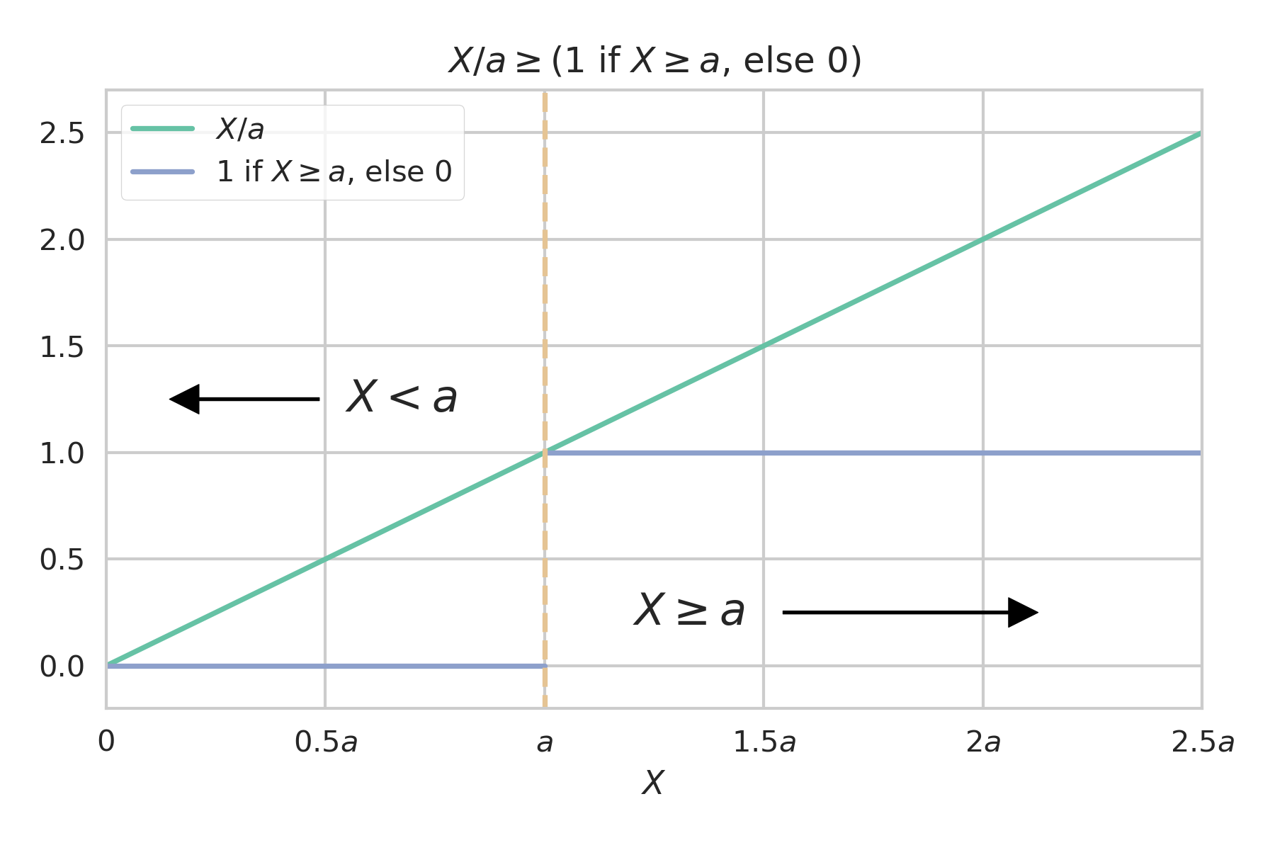
We can immediately see that

holds for all values of $X$ (keeping in mind that $X$ and $a$ are both constrained to be non-negative). It’s also important to note that the line defined by $\frac X a$ couldn’t possibly be lowered any further without violating this inequality because the two functions touch at $(0,0)$ and $(a,1)$. We could increase the slope or add some constant to $\frac X a$ and it would still be greater than or equal to the piece-wise function, but if our goal is to put a bound on the expectation value then we naturally want the bound to be as tight as possible. The choice of $\frac X a$ seems less arbitrary when you think of it as the tightest linear bound that can be placed on the piece-wise function.

Now, given that $\frac X a$ is greater than or equal to the piece-wise function for all $X$, it follows that the expectation values also follow this inequality.

Plugging this back into our prior expression for $\mathbb P(X \geq a)$ allows us to reproduce Markov’s inequality.

This amounts to a proof of the inequality, but the relationship itself might not seem particularly intuitive yet. When thinking about these type of inequalities, I often find it helpful to think about how far different distributions will fall from equality and to look at the most extreme distributions that prevent the bounds from being any tighter.

We already saw that $\frac X a$ and the piece-wise function are identical at only $X=0$ and $X=a$. This means that the equality will only hold for distributions that have finite probability at only those two points. The size of the contribution to inequality will grow linearly as a function of $X$ from $0$ until $a$, where it will drop back to zero and then continue growing linearly off to infinity. We can see then that probability distributions with high densities at $X \gg a$ would be furthest from equality. On the other hand, if most of the probability density is centered around $a$ then it’s going to be the portion of the distribution where $X$ is just less than $a$ that contributes most significantly.

These interpretations can be made more clear by taking a look at how close specific distributions come to the bound. A convenient set of distributions to use for this purpose are $\chi^2$ distribution with different degrees of freedom $k$. A $\chi^2$ distribution is defined as

for $X \geq 0$ and describes the distribution of the sum of the squares of $k$ normally distributed independent random variables with $\mu=0$ and $\sigma=1$. If we scale $X$ by a factor of $k$ then we get the distribution for the mean of the $k$ random variables squared rather than the sum. This is nice because it keeps each distribution centered at $1$ while the peaks grow increasingly narrow for large $k$.

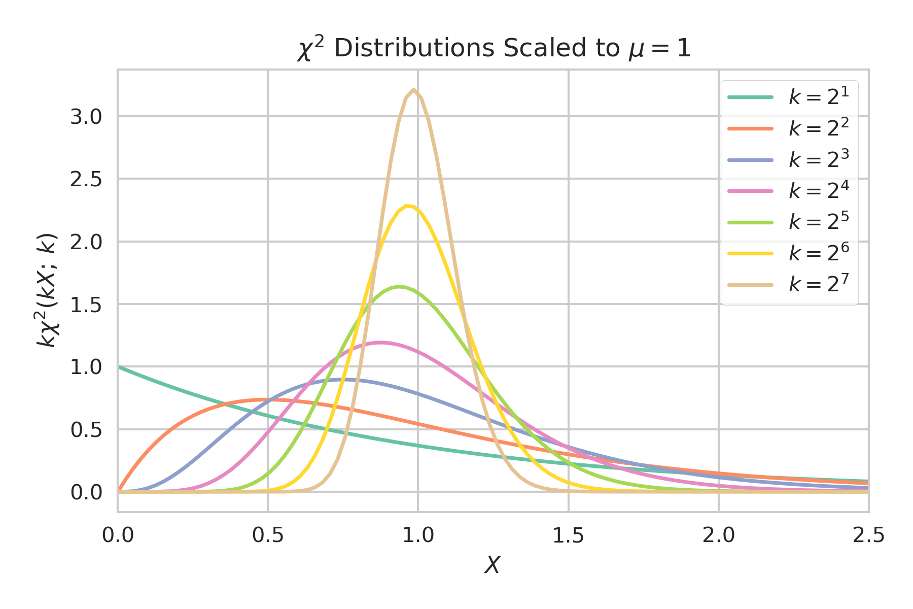
One thing that we can notice here is that values of $a \gg 1$ will be close to the bound because the bulk of the distributions will fall relatively close to zero and the contributions resulting from $\frac X a > 0$ will be small. The distributions will also become close to the bound for large $k$ when $a$ is slightly less than $1$ because the probability will be densely focused at $X$ just greater than $a$ where the contributions from $\frac X a > 1$ will be small. Increasing $a$ to be slightly more than $1$ will quickly cause the bound to become much looser as $\frac X a \approx 1$ is now being compared to $0$ instead of $1$.

This plot shows how close the various scaled $\chi^2$ distributions come to the bounds for different values of $a$.

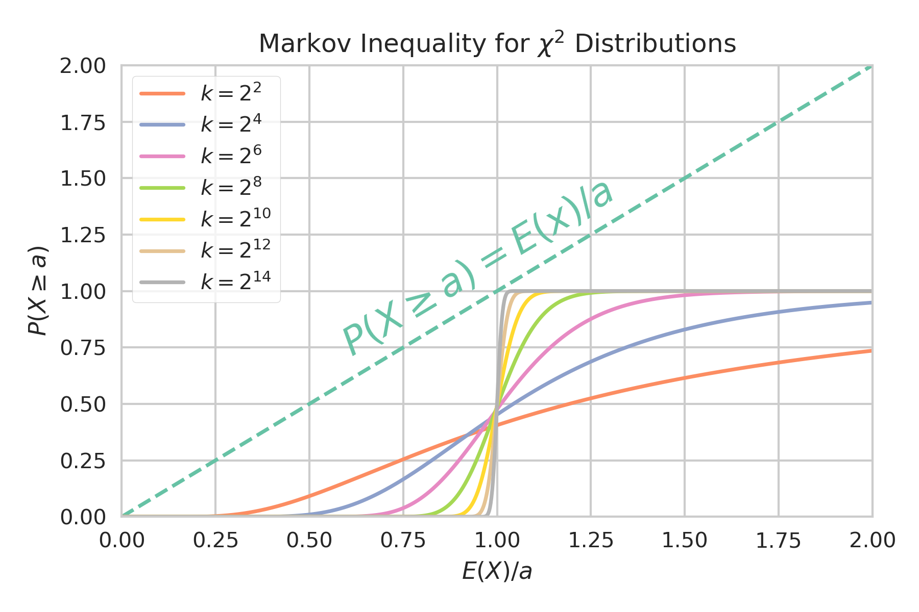
Keep in mind that the $x$-axis here is $\frac {\mathbb E(X)} a$ so large values of $a$ are actually to the left of the plot. We can see that for very large values of $a$, the curves all intercept the bound at $0$ as we suspected. The more interesting feature is how the curves get progressively closer to the bound for larger $k$ and how the near intercept is happening at $a$ just less than $\mathbb E(X) = 1$. This also matches what we predicted, as does the fact that the curves quickly move away from the bound as $a$ grows above $1$.

Chebyshev’s Inequality

After understanding Markov’s inequality, it’s actually fairly trivial to get Chebyshev’s inequality. Recall that Chebyshev’s inequality relates to what fraction of a probability distribution falls more than some distance from its mean. This can be expressed as $\mathbb P(|X-\mu| \geq a)$ which is equivalent to $\mathbb P((X-\mu)^2 \geq a^2)$. Treating $(X-\mu)^2$ as a new non-negative random variable allows us to apply Markov’s Inequality to find that $\mathbb P((X-\mu)^2 \geq a^2) \leq \mathbb E((X-\mu))^2)/a^2 = \sigma^2/a^2$. If we now define $k=a/\sigma$ then we immediately get Chebyshev’s Inequality.

This gives us a limit on how much of a distribution could possibly fall outside of some number of standard deviations from the mean. For example, the fraction of the distribution that can fall outside of two standard deviations must be less than $1/{2^2} = 0.25$. This is quite a bit more than than the $\sim 0.05$ that the 68-95-99.7 rule would suggest for a normal distribution, but this simply means that it as a very loose bound in that circumstance.

Just as with Markov’s inequality, I find that understanding the distributions for which the bounds of Chebyshev’s inequality are particularly tight is helpful for developing intuition around it and its extensions. We basically just applied Markov’s inequality to a random variable $(X-\mu)^2$ and so the same conditions for the bounds being sharp apply here. In other words, equality will only hold for distributions with non-zero probability only at values of $X$ satisfying $(X-\mu)^2=0$ and $(X-\mu)^2=a^2=k^2 \sigma^2$. $X$ can therefore only take on values at $\mu$, $\mu + k\sigma$, or $\mu - k\sigma$. We can parameterize the set of probability distributions where Chebyshev’s inequality would be sharp as

where $\alpha$ and $\beta$ determine the relative probabilities at the three allowed points.

When we were dealing with Markov’s inequality, it didn’t matter how much of the distribution was centered at $X=0$ relative to at $X=a$. Both points corresponded to the inequality being tight and we saw that a distribution could be close to the bound if either $a$ extended far beyond the bulk of the distribution or if the distribution was tightly peaked just above $a$. The situation is slightly more complicated with Chebyshev’s inequality because the locations of the allowed points are expressed in terms of the mean and standard deviation. If we were to give the points relative probabilities that would result in $\mu$ not equaling the mean or $\sigma$ not equaling the standard deviation, then we would have created a contradiction and we would know that something must be wrong. We have to instead be careful that our choices of $\alpha$ and $\beta$ do not result in any contradictions or violations of our initial assumptions.

Let’s start by requiring that $\mu = \mathbb E(X)$ as we would expect.

This tells us that the contributions from the two points separated from the mean by $k\sigma$ on either side must be equal. If this weren’t the case then the side with a higher probability would pull the mean towards it so that it would no longer be centered at $\mu$.

We can now apply the same logic with respect to the variance by requiring that $\sigma^2 = \mathbb{E} \left( (X - \mu)^2 \right )$.

This tells us that the probability for each of the two points where $|X-\mu| \geq k\sigma$ are equal to exactly half of the maximum amount that Chebyshev’s equality allows, $\frac 1 {k^2}$. We couldn’t really expect these to have any other value considering that we’ve specifically constructed the distribution to exactly meet this bound.

Finally, we can use the normalization to find $\alpha$.

Now that we’ve constrained both parameters, we can rewrite the probability distribution using these exact weights.

The point at $X = \mu$ can be thought of as pulling the standard deviation downwards while the points at $X = \mu \pm k\sigma$ pull it upwards (assuming $k > 1$). To maximize $\mathbb P(|X - \mu| \geq k\sigma)$, it makes sense that we would want the distribution inside of the bound to reduce the standard deviation as much as possible while the distribution outside of the bound should increase the standard deviation as little as possible. This is exactly what we see with $X = \mu$ being the optimal location to reduce the standard deviation while $X = \mu \pm k\sigma$ are the optimal locations for increasing it as little as possible while also satisfying $|X - \mu| \geq k\sigma$. The relative probabilities between these must then balance each other such that the standard deviation equals exactly $\sigma$. It’s only natural that the resulting combined probability for $X = \mu \pm k\sigma$ gives you the exact maximum value for $\mathbb P(|X - \mu| \geq k\sigma)$ that Chebyshev’s inequality would allow.

One consequence of this is that a distribution for which Chebyshev’s inequality is a relatively tight bound will tend to have a distinct three peaked structure with the two outside peaks falling just beyong $X = \mu \pm k\sigma$. If you encounter a distribution that appears to be unimodal then you can safely suspect that $\mathbb P(|X - \mu| \geq k\sigma)$ is less than the bound suggested by Chebyshev’s inequality. By introducing the restriction that a distribution is unimodal, you can actually explicitly show that the bound is reduced by a factor of $\frac 4 9$ giving the Vysochanskiï–Petunin inequality. There are also countless other related inequalities, all following the same basic idea, but relying on slightly different assumptions about symmetry, the number of modes, distribution bounds, etc.

The Law of Large Numbers

I find that Chebyshev’s inequality can be helpful when making rough estimates about confidence intervals, but it’s also often a very useful tool when proving things in statistics. One simple, but important proof, where Chebyshev’s inequality is often used is that of the law of large numbers. Let’s quickly walk through that proof to see a concrete example of how the inequality can be applied.

The law of large numbers states that for $k$ independent and identically distributed random variables, $X_1,X_2,\dots,X_k$, the sample mean

converges to the expected value $\mu$ as $k \to \infty$. Before getting to the proof, let’s take an empirical look at how the sample mean converges.

Consider the case where $X$ is distributed according to $\sqrt{X} \sim \mathcal{N} (0,1)$. The sample mean here will be equivalent to the average of the square of $k$ normally distributed random variables with $\mu=0$ and $\sigma=1$. By tracing the sample means as the sample size grows for $100$ distinct samples, we can see how the sample means all begin to converge towards a value of $1$.

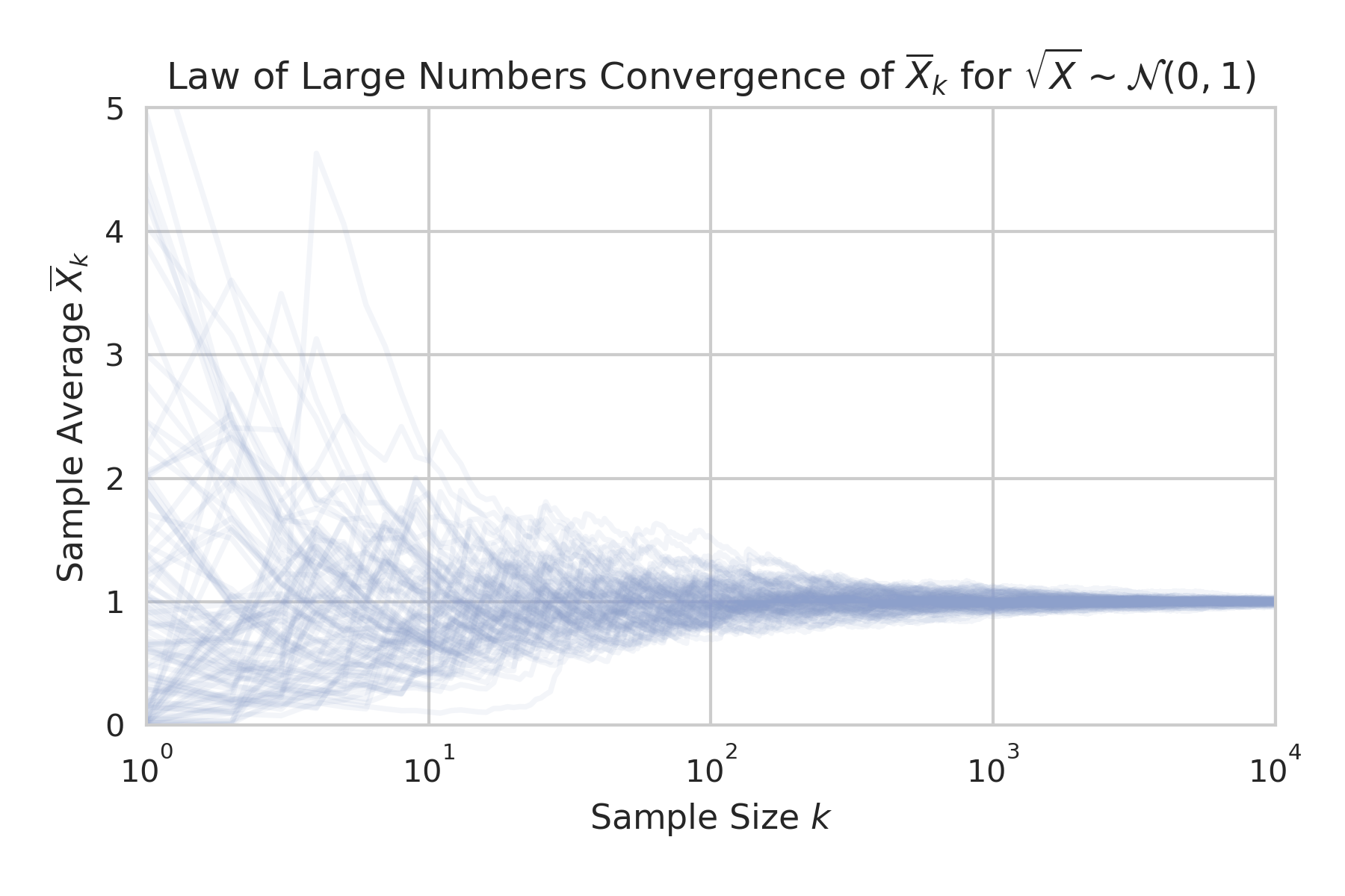
We could have done the same thing for the sample mean of a normally distributed random variable instead of the square of a normally distributed random variable, but this choice lets us connect this plot back to some of what we did earlier. When $X$ is distributed according to $\sqrt{X} \sim \mathcal{N} (0,1)$ then the sample mean of $X$ will be distributed according to ${\overline X}_k \sim k \cdot \chi^2 \left(k \cdot {\overline X}_k;,k \right)$. This is precisely the scaled $\chi^2$ distribution that we used earlier to explore the tightness of the bound from Markov’s inequality. Each scaled $\chi^2$ distribution that we plotted before describes the distribution of sample means here at the corresponding value of $k$. This isn’t particularly more relevant to the law of large numbers or anything, but this connection might help to clarify the meaning of those distributions if you weren’t totally clear on where they came from earlier.

Getting back to the proof, we’ll first want to find the expectation values for both the sample mean and its variance. Beginning with the sample mean, we find that

It’s a bit hard to imagine how the sample mean could be anything but $\mu$, but it’s nice to see this explicitly. Similarly, we can compute the variance of the sample mean as

This is mostly basic algebraic manipulation, but I should point out that the covariances are all equal to zero because of the whole independent and identically distributed assumption. It’s also worth emphasizing that the variance of the sample mean does not simply equal $\sigma^2$, instead carrying an additional factor of $\frac 1 k$. This is one of the most commonly used facts in all of statistics, and it’s really at the heart of why the law of large numbers is true.

At this point, we’ve shown that the distribution of $\overline X_k$ has a mean of $\mu$ and a standard deviation of $\frac{\sigma}{\sqrt{k}}$ that will approach zero as $k$ goes to infinity. This strongly suggests that the sample mean is going to converge to $\mu$ at large $k$, but we have to be certain that there can’t be a meaningful number of outliers even as the standard deviation gets arbitrarily small. That’s where Chebyshev’s inequality comes into play.

For any arbitrarily small positive number $\epsilon$, we can use Chebyshev’s inequality to show that the probability that the sample mean falls outside of a distance $\epsilon$ from $\mu$ is

which implies that the probability of the sample mean falling within $\epsilon$ of $\mu$ is

This probability approaches $1$ as $k$ goes to infinity and so the sample mean converges in probability to $\mu$

This proof might feel a bit laborious for something that seems obvious, but there are actually some subtleties that come into play and justify the attention to detail. For example, we showed that the sample mean converges in probability to $\mu$ while the stronger statement that it converges almost surely to $\mu$ can also be proven. These two different types of convergence correspond to the weak and strong forms of the law of large numbers and we only proved the weak form. The details of this are a bit out of scope for this article, but you can read about convergence of random variables if you would like to learn more.

Conclusion

Hopefully you were able to find this helpful in terms of developing intuition around inequalities involving random variables. Even if you were already familiar with Markov’s and Chebyshev’s inequalities, you may not have put much thought into the distributions that result in sharp bounds. I find that having a good mental picture for how different parts of a distribution contribute to the tightness of an equality allows me to do a better job of making rough estimates for things. For example, combining an understanding of Chebyshev’s and the Vysochanskij–Petunin inequality with the 68-95-99.7 rule makes it possible to give reasonable ballpark estimates of confidence values by eye.

If your company has a lot of data and is looking to extract value out of it, please don’t hesitate to get in touch. Whether you’re trying to make more accurate suggestions for your users or just to improve your conversion rates, Intoli can absolutely help you get the results you want.