Understanding Neural Network Weight Initialization

By Andre Perunicic | July 25, 2017

Choosing Weights: Small Changes, Big Differences

There are a number of important, and sometimes subtle, choices that need to be made when building and training a neural network. You have to decide which loss function to use, how many layers to have, what stride and kernel size to use for each convolution layer, which optimization algorithm is best suited for the network, etc. With so many things that need to be decided, the choice of initial weights may, at first glance, seem like just another relatively minor pre-training detail, but weight initialization can actually have a profound impact on both the convergence rate and final quality of a network.

In order to illustrate this fact, I’ve trained the same neural network using three different weight initialization strategies and plotted the results in Figure 1. (You can find code for generating the plots featured in this article in our article materials GitHub repository.) Each subplot displays the 10-batch rolling average of the loss attained while training a basic convolutional neural network that classifies handwritten digits. The training set consists of 60000 digit scans comprising the famous MNIST dataset. The network was trained for 12 epochs with a batch size of 128 images for each weight initialization strategy.

MNIST CNN Losses

Figure 1: *Training loss of a simple CNN over 12 epochs. The middle line represents the 10 batch rolling average over 12 epochs, while the error bands show variability around this mean.*

In the leftmost case, all weights are initially set to zero and the network can’t learn at all. The middle plot shows weights drawn from a normal distribution with a standard deviation of 0.4. Loss does improve over time, but the rate of convergence is very low and the network barely achieves a validation accuracy of about 88% in 12 epochs. In the rightmost plot, the weights are drawn from normal distributions with variances which are inversely proportional to the number of inputs into each neuron. With a final loss two orders of magnitude smaller than in the other two cases and a validation accuracy greater than 99%, this strategy is the clear winner.

But why does this happen in the first place and how can you choose the right initial weights for your network? TensorFlow, Keras, and most neural network libraries come with a host of sane choices out of the box, but where do they come from? What’s up with that $ \sqrt{6} $ factor anyway? In this post I’ll explore the effects of initial weight selection strategies and how to make some sense of these results. After reading the article, you should be able to make an informed decision about weight initialization in your own networks.

Information Flow in a MLP

One way to evaluate what happens under different weight initializations is to visualize outputs of each neuron as a dataset passes through the network. In particular, we’ll compare the outputs of subsequent layers of a Multi-Layer Perceptron (MLP) under different initialization strategies.

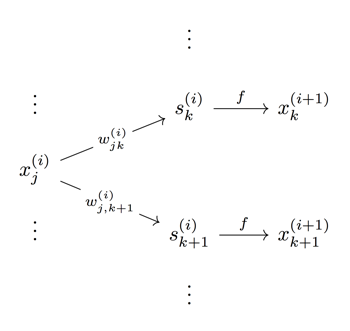
An $(M+1) $-layer MLP is the network that has an input layer, $M $ fully-connected “hidden” layers, and an output layer. The $i$-th hidden layer accepts the previous layer’s outputs as a $ n_i $-dimensional input vector $x^{(i)}$, applies a linear transformation $W^{(i)}$ to this vector to get an intermediate vector $s^{(i)}$, and finally applies a non-linear activation function such as $\tanh(s) $ or $\text{ReLU} = \max(0, s) $ to each entry of $s^{(i)}$ to get the current layer’s activations or outputs that are passed onwards.

In other words, if $ x^{(i)} = (x_1^{(i)}, \ldots, x_{n_i}^{(i)}) $ denotes the outputs of layer $ i $ (with $ i = 0 $ corresponding to the input layer), then layers are related via

\[ x^{(i+1)} = f(x^{(i)} W^{(i)})\,, \]

where $f $ is an activation function operating on each entry of the vector $s^{(i)} = x^{(i)} W^{(i)} $ and $W^{(i)} $ is the $n_i \times n_{i+1} $ matrix of weights connecting layers $i $ and $i+1 $.

Per-entry this formula is written as

\[ \begin{align*} x^{(i+1)}_{a} &= f(x^{(i)}W^{(i)}_{\bullet, a}) \\ &= f(x^{(i)}_1 w^{(i)}_{1a}+\ldots +x_{n_i}^{(i)}w^{(i)}_{n_ia} ) \end{align*} \]

for each $a \in \{ 1 \ldots n_{i+1} \} $, with $W^{(i)}_{\bullet, a}$ denoting the $a$-th column of $W^{(i)}$. Figure 2 summarizes the MLP as a diagram.

\[ x^{(0)} \xrightarrow {W^{(0)}} \underbrace{\left( s^{(0)} \xrightarrow{f} x^{(1)} \right)}_{\text{Hidden Layer 1}} \xrightarrow{W^{(1)}} \ldots \xrightarrow{W^{(M-1)}} \underbrace{\left( s^{(M-1)} \xrightarrow{f} x^{(M)} \right)}_{\text{Hidden Layer M}} \xrightarrow{W^{(M)}} \underbrace{ \left( s^{(M)} \xrightarrow{\sigma} \sigma(s^{(M)}) \right) }_{\text{Output Layer}} \]

Figure 2: *Diagrammatic view of a multi-layer perceptron.*

The final output layer won’t be featured too prominently in what follows, but for completeness, I’ll just mention that it simply takes the last hidden layer’s activations and mashes them together into one or more outputs $s_a^{(M)} = \sum_j x_j^{(M)} w_{ja}^{(M)} $ which can be compared to training data in order to learn the network’s weights. In a binary classification setting, for instance, one would typically pass a single $s^{(M)} $ variable through a sigmoid $\sigma $ to interpret $s^{(M)} $ as a “score” and the final output $\sigma(s^{M}) $ as a classification probability. One also typically adds a bias term to the activations $s^{(i)} $, but I’ll omit them since they are not instrumental for the purposes of this article.

The MLP under consideration here features $M = 5$ hidden layers with $n_i = 100 $ neurons each and receives normalized and flattened MNIST images as input. Let’s first consider trivial activation functions $f(s) = s $. Doing so causes the network to become a sequence of linear transformations. This may at first seem like a silly thing to do since neural networks derive much of their usefulness from being nonlinear. However, results produced in the linear regime often yield outcomes that are “good enough” in the nonlinear case, or which can be adapted to nonlinear activation functions with a little bit of tweaking.

Output Progression in a Linear Network

Figure 3: *Activations of each hidden layer of a MLP after one forward pass through the network.*

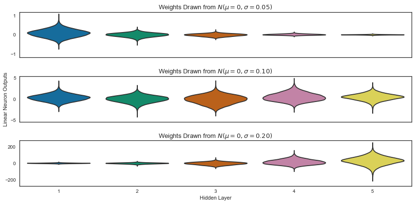
Each subplot of Figure 3 shows activations of hidden layers after one batch of 1000 MNIST images are passed through the MLP. There are three subplots because we are considering three distinct initialization strategies for $W^{(i)} $. Note that each subplot is on its own scale in order to show outputs relative to the first hidden layer.

Top: The weights are drawn from a zero centered Gaussian with standard deviation $\sigma = 0.05 $. Here the activations quickly dwindle to almost nothing.
Middle: The weights are drawn from a zero centered Gaussian with standard deviation $\sigma = 0.1 $. The distribution of activations retains its shape throughout the network.
Bottom: The weights are drawn from a zero centered Gaussian with standard deviation $\sigma = 0.2 $. This time the activations become increasingly spread out as we progress through the network.

Vanishing or diverging activations, as in the top and bottom cases of Figure 3, are an impediment for efficiently training a neural network. Let’s understand why this is the case by examining how information flows through a network during training.

Neural networks are typically trained by minimizing a loss function $L(W) $ with respect to the weights using gradient descent. That was kind of mouthful so let me quickly remind you what it means. Weights of a neural network are the “variables” of the function $L$. The loss depends on the dataset, but only implicitly: it is typically the sum over each training example, and each example is effectively a constant. Training just means moving around the weight space (i.e., choosing different weights) until we find a set for which the loss – our measure of failure – is as low as possible. Since the gradient of any function always points in the direction of steepest increase, all we have to do is calculate the gradient of $L$ with respect to the weights $W$ and move in the opposite direction a little bit, then rinse and repeat.

There is nothing particularly deep about this method, but to make the calculation efficient we have to calculate the gradient quickly. This is possible due to the backpropagation algorithm which enables calculating $\nabla L $ in stages, courtesy of the chain rule from calculus. The chain rule states that to calculate the rate of change of a function $L$ with respect to one of its variables $w_{jk}^{(i)}$ (the partial derivative of $L$ with respect to $w_{jk}^{(i)}$ we can calculate the derivative with respect to a higher-level variable $x_k^{(i+1)}$ which depends on $w_{jk}^{(i)}$ first, then multiply it by the derivative of $x_k^{(i+1)}$ with respect to $w_{jk}^{(i)}$. Mathematically, for the particular case of a neural network like the MLP, that can be written as

\[ \frac{\partial L}{\partial w_{jk}^{(i)}} = \frac{\partial L}{\partial x_k^{(i+1)}} \frac{\partial x_k^{(i+1)}}{\partial w_{jk}^{(i)}}\,. \]

The first term on the right can be computed recursively, as we will see below. The second term on the right is the only place directly involving the weight $w_{jk}^{(i)} $ and can be broken down into

\[ \begin{align*} \frac{\partial{x_k^{(i+1)}}}{\partial w_{jk}^{(i)}} &= \frac{\partial{f(s^{(i)}_j)}}{\partial s_j^{(i)}} \frac{\partial s_j^{(i)}}{\partial w_{jk}^{(i)}} \\ &=f'(s^{(i)}_j)\, x_j^{(i)}. \end{align*} \]

From this you can see that if the outputs tend to zero the gradients do as well, which causes the weights to stop updating. On the other hand, if $s_j^{(i)} $ end up being too extreme, the activations $f $ could have zero derivatives and again prevent the weights from updating.

All this suggests that the aim should be to maintain variance of activations throughout the network, since then we avoid the two extreme situation highlighted above. How can weight initialization help us achieve this goal? For an activation function such as $f(s) = s $ or $f(s) = \tanh(s) $ satisfying $f'(s) \approx 1 $ near zero we can approximate how variance of the outputs depends on the variance of the weights and the inputs as we move forward and backward through the network.

Local View of a Neural Network Node

Figure 4: *A local view of the `$x_j^{(i)} $` node.*

Going forward we have

\[ x_k^{(i+1)} \approx \sum_{j = 1}^{n_i} x_j^{(i)} w_{jk}^{(i)}\,. \]

Assuming that the weights and activations of each layer vary jointly per layer and that their means are zero, we can use basic properties of variance to express the variance of the $(i+1)$-th layer’s outputs in terms of the variances of the $i$-th layer’s weights and outputs:

\[ \begin{align*} \text{Var}(x^{(i+1)}) & \approx \text{Var} \left( \sum_{j = 1}^{n_i} x_j^{(i)} w_{jk}^{(i)} \right) \\ & \approx \sum_{j=1}^{n_i} \text{Var}( x^{(i)} ) \text{Var}( w^{(i)} )\,. \end{align*} \]

This then simplifies to

\[ \text{Var}(x^{(i+1)}) = n_i \text{Var}(x^{(i)}) \text{Var}(w^{(i)}) \]

In order to achieve $\text{Var}(x^{(i+1)}) = \text{Var}(x^{(i)}) $ we therefore have to impose the condition

\[ \text{Var}( w^{(i)}) = \frac{1}{n_i}\,. \]

On the other hand, the multivariate chain rule states that to compute the derivative of $L$ with respect to $ x_j^{(i)}$, we can add up the contributions coming from the variables $ x_k^{(i+1)}$ through which there is a direct path to $L$. If we denote $\frac{\partial L}{\partial x_j^{(i)}} $ by $\Delta_j^{(i)} $ this can be formally written as

\[ \begin{align*} \Delta_j^{(i)} \equiv \frac{\partial L}{\partial x_j^{(i)}} & = \sum_{k=1}^{n_{i+1}} \frac{\partial L}{\partial x_k^{(i+1)}} \frac{\partial x_k^{(i+1)}}{\partial x_j^{(i)}}\\ & = \sum_{k=1}^{n_{i+1}} \frac{\partial L}{\partial x_k^{(i+1)}} f'(s_j^{(i)}) w_{jk}^{(i)}\,, \end{align*} \]

Assuming that $f'(s_j^{(i)}) \approx 1 $ and calculating variance as before, we obtain the relation

\[ \text{Var}(\Delta^{(i)} ) = n_{i+1} \text{Var}(\Delta^{(i+1)}) \text{Var}(w^{(i)})\,. \]

This means that we should also impose the condition

\[ \text{Var}(w^{(i)}) = \frac{1}{n_{i+1}}\,. \]

Unless $n_i = n_{i+1} $, we have to compromise between these two conditions, and a reasonable choice is the harmonic mean

\[ \text{Var}(w^{(i)}) = \frac{2}{n_i+n_{i+1}}\,. \]

If we sample weights from a normal distribution $N(0, \sigma) $ we satisfy this condition with $\sigma = \sqrt{\frac{2}{n_i + n_{i+1}}} $. For a uniform distribution $U(-a, a) $ we should take $a = \sqrt{\frac{6}{n_i+n_{i+1}}} $ since $\text{Var} \left( U(-a,a) \right) = a^2/3 $. We have thus arrived at Glorot initialization. This is the default initialization strategy for dense and 2D convolution layers in Keras, for instance.

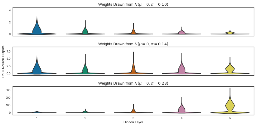
Glorot initialization works pretty well for trivial and $ \tanh $ activations, but doesn’t do as well for $ \text{ReLU} $. Luckily, since $ f(s) = \text{ReLU}(s) $ just zeroes out negative inputs, it roughly removes half the variance and this is easily amended by multiplying one of our conditions above by two:

\[ \text{Var}(w^{(i)}) = \frac{2}{n_i}\,. \]

It may also be worth nudging the weights a bit away from zero towards a positive mean when using $ \text{ReLU} $ activations, since derivatives are zero for negative numbers. For a more formal treatment of this idea, you can check out the He initialization paper.

ReLU Output Progression

Figure 6: *Output progression for $\text{ReLU}$ activations. Note that this time `$\sigma = 0.14 \approx \sqrt{2/100}$` preserves variance across the network.*

Other Approaches

Some approaches incorporate variance scaling directly into the network architecture. This is an active area of research – see, for example, this paper about self-normalizing neural networks from June – but a simple to use technique that has gained a lot of popularity is batch normalization. The basic idea is to insert extra layers that normalize data after fully-connected and convolutional layers in your network. This optimizes the data flow dynamically, which allows the network to achieve good results with a wider range of initialization strategies. Given that the added layers are compatible with backpropagation, the technique is essentially plug-and-play so the most obvious downside is a small runtime penalty due to the extra layers.

Yet another approach is to initialize the network based on a pre-training data analysis step (there is both a paper and a code repository about this if you’d like to know more). Architectures like ResNet encourage data flow by including connections that skip layers. As a final example of this principle, LSTMs also prevent output degradation with explicit memory cells.

In the zoo of techniques that are modern neural networks, there is a new approach just around the corner even for seemingly simple matters like weight initialization. If you need assistance with your own network architectures or want advanced analytics integrated into your crawls, we are here to help. Just get in touch!