Introduction

Principal Component Analysis, or PCA, is a well-known and widely used technique applicable to a wide variety of applications such as dimensionality reduction, data compression, feature extraction, and visualization. The basic idea is to project a dataset from many correlated coordinates onto fewer uncorrelated coordinates called principal components while still retaining most of the variability present in the data.

Singular Value Decomposition, or SVD, is a computational method often employed to calculate principal components for a dataset. Using SVD to perform PCA is efficient and numerically robust. Moreover, the intimate relationship between them can guide our intuition about what PCA actually does and help us gain additional insights into this technique.

In this post, I will explicitly describe the mathematical relationship between SVD and PCA and highlight some benefits of doing so. If you have used these techniques in the past but aren’t sure how they work internally this article is for you. By the end you should have an understanding of the motivation for PCA and SVD, and hopefully a better intuition about how to effectively employ them.

Encoding Data as a Matrix

Before we discuss how to actually perform PCA it will be useful to standardize the way in which data is encoded in matrix form. Since PCA and SVD are linear techniques, this will allow us to manipulate the data using linear transformations more easily.

It’s simplest to start with an example, so suppose that you are given the width $w$, height $h$, and length $l$ measurements of $n = 1000$ rectangular boxes. We can encode the measurements of box $i$ as a $(w_i, h_i, l_i)$ tuple called a sample. Each sample is a vector in $d = 3$ dimensions, since there are 3 numbers describing it. Because vectors are typically written horizontally, we transpose the vectors to write them vertically:

To pack the data into a single object we simply stack the samples as rows of a data matrix,

The columns of this matrix correspond to a single coordinate, i.e., all the measurements of a particular type.

In the general case, we are working with a $d$-dimensional dataset comprised of $n$ samples. Instead of using letters like $h$, $w$, and $l$ to denote the different coordinates, we simply enumerate the entries of each data-vector so that $x_i^T = (x_{i1}, \ldots, x_{id})$. Before placing these vectors into a data matrix, we will actually subtract the mean of the data

from each sample for later convenience. We then use these zero-centered vectors as rows of the matrix

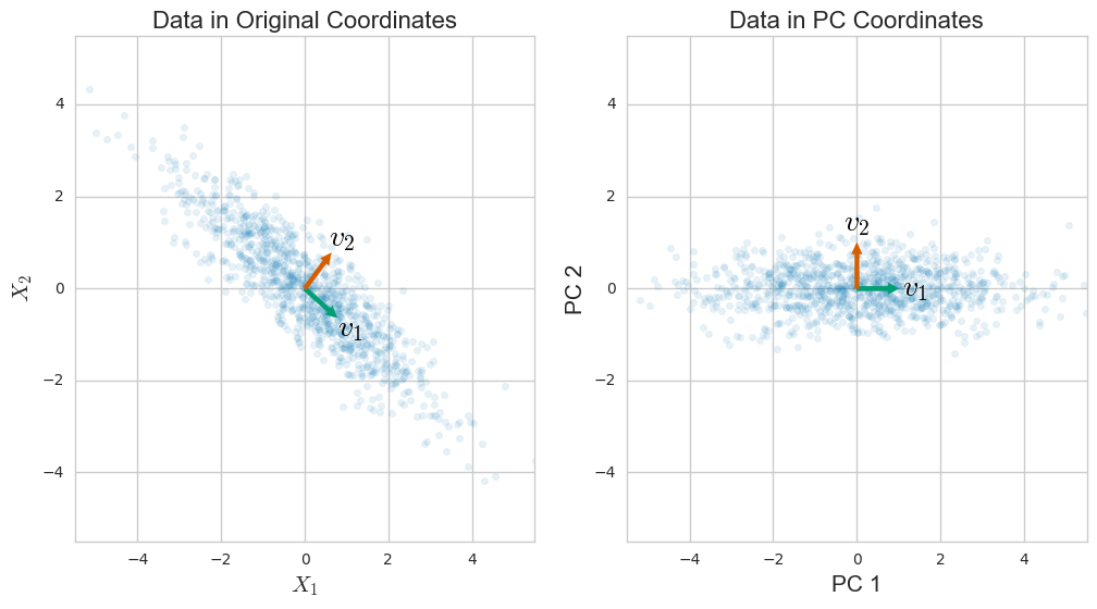
See Figure 1 for a visual illustration of the case $n = 1000$, $d = 2$. Placing data into a matrix is particularly convenient because it allows us to write the sample covariance around the mean using matrices as

Dividing by $n - 1$ is a typical way to correct for the bias introduced by using the sample mean instead of the true population mean. The covariance matrix will take center stage as we work through understanding principal components and singular value decomposition.

Principal Component Analysis

One of the first papers to introduce PCA as its known today was published in 1933 by Hotelling. The author’s motivation was to transform a set of possibly correlated variables into “some more fundamental set of independent variables … which determine the values [the original variables] will take.” Coming from psychology, his first choice for naming them was “factors,” but given that this term already had a meaning in mathematics he called the reduced set of variables “components” and the technique to find them “the method of principal components.” These components are chosen sequentially in a way that lets their “contributions to the variances of [the original variables] have as great a total as possible.”

Mathematically, the goal of Principal Component Analysis, or PCA, is to find a collection of $k \leq d$ unit vectors $v_i \in \mathbb R^d$ (for $i \in {1, \ldots, k }$) called Principal Components, or PCs, such that

1. the variance of the dataset projected onto the direction determined by $v_i$ is maximized and
2. $v_i$ is chosen to be orthogonal to $v_1, \ldots, v_{i-1}$.

Now, the projection of a vector $x \in \mathbb R^d$ onto the line determined by any $v_i$ is simply given as the dot product $v_i^T x$. This means that the variance of the dataset projected onto the first Principal Component $v_1$ can be written as

To actually find $v_1$ we have to maximize this quantity, subject to the additional constraint that $\| v_1 \|= 1$. Solving this optimization problem using the method of Lagrange multipliers turns out to imply that

which just means that $v_1$ is an eigenvector of the covariance matrix $S$. In fact, since $\| v_1 \| = v_1^T v_1 = 1$ we also conclude that the corresponding eigenvalue is exactly equal to the variance of the dataset along $v_1$, i.e.,

You can continue this process by projecting the data onto a new direction $v_2$ while enforcing the additional constraint that $v_1 \perp v_2$, then onto $v_3$ while enforcing $v_3 \perp v_1, v_2$, and so on.

The end result is that the first $k$ principal components of $X$ correspond exactly to the eigenvectors of the covariance matrix $S$ ordered by their eigenvalues. Moreover, the eigenvalues are exactly equal to the variance of the dataset along the corresponding eigenvectors.

You may have noticed that this result suggests that there exists a full set of orthonormal eigenvectors for $S$ over $\mathbb R$. Indeed, since $S$ is a real symmetric matrix, meaning that $S = S^T$, the Real Spectral Theorem implies exactly that. This is a non-trivial result which we will make use of later in the article, so let’s expand on it a little bit. Consider the case of $k = d < n$. Taking $k = d$ principal components may seem like a strange choice if our purpose is to understand $X$ through a lower dimensional subspace, but doing so allows us to construct a $d \times d$ matrix $V$ whose columns are the eigenvectors of $S$ and which therefore diagnoalizes $S$, i.e.,

where $\Lambda = \text{diag}(\lambda_1, \ldots, \lambda_d )$ and $r = \text{rank}(X)$. In other words, the principal components are the columns of a rotation matrix and form the axes of a new basis which can be thought of as “aligning” with the dataset $X$. Of course, this image works best when $X$ is blobby or looks approximately normal.

Singular Value Decomposition

Singular Value Decomposition is a matrix factorization method utilized in many numerical applications of linear algebra such as PCA. This technique enhances our understanding of what principal components are and provides a robust computational framework that lets us compute them accurately for more datasets.

Let’s start with a review of SVD for an arbitrary $n \times d$ matrix $A$. SVD is motivated by the fact that when viewed as a linear transformation, $A$ maps the unit sphere $\mathbb S^d \subset \mathbb R^d$ to a (hyper)ellipse in $\mathbb R^n$. Let’s consider an example with $n = d = 2$ in order to more easily visualize this fact.

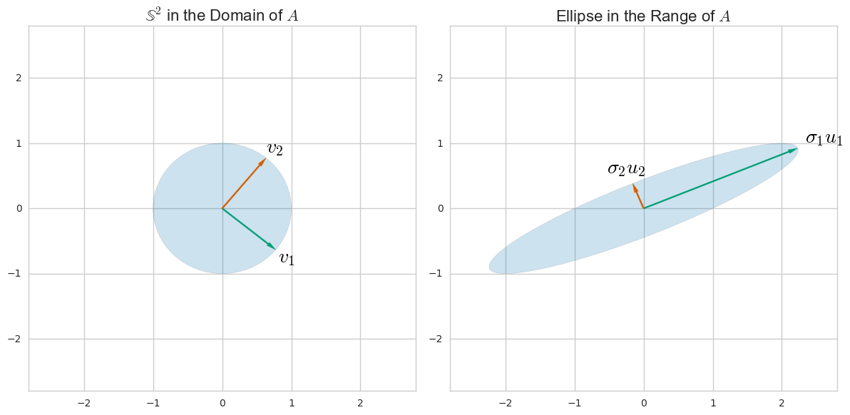
From this figure we can extract a few useful definitions which hold for arbitrary dimensions with a few extra caveats:

• The lengths $\sigma_i$ of the semi-axes of the ellipse $A\mathbb S^d \in \mathbb R^n$ are the singular values of $A$.
• The unit vectors ${ u_i }$ along the semi-axes of the ellipse are called the “left” singular vectors of $A$.
• The unit vectors $v_i$ such that $Av_i = \sigma_i u_i$ are called the “right” singular vectors of $A$.

Proving the existence and uniqueness of the singular values and singular vectors is a bit beyond the scope of this article, but the proof is relatively straightforward and can be found in any book on numerical linear algebra (see below for a reference). The two-dimensional image in Figure 2 hopefully provides enough guidance for the result to be intuitive, however.

What may not be immediately apparent from the picture is that depending on $n, d$ and $r = \text{rank}(A)$, some of the left singular vectors may “collapse” to zero. This happens when the matrix $A$ does not have full rank for instance, since then its range must be a subspace of $\mathbb R^n$ with dimension $r < d$. In general, there are exactly $r = \text{rank}(A)$ singular values and the same number of left singular vectors.

By stacking the vectors $v_i$ and $u_i$ into columns of matrices $\widehat V$ and $\widehat U​$, respectively, we can write the relations $Av_i = \sigma_i u_i$ as

where $\widehat \Sigma = \text{diag}(\sigma_1, \ldots, \sigma_r)$. By padding $\widehat \Sigma$ with zeros and adding arbitrary orthonormal columns to $\widehat U$ and $\widehat V$ we obtain a more convenient factorization

Since $V$ is unitary – that is, it has unit length, orthonormal columns – it follows that $V^{-1} = V^T$, so multiplying by $V^T$ gives us the singular value decomposition of $A$:

Things got a bit busy here, so here’s a visual summary of this result.

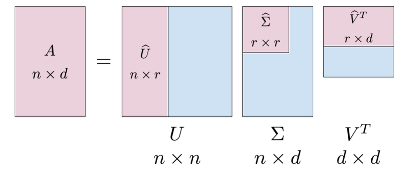
Note that this result is in the end consistent with the ellipse picture above since the effect of the three transformations is to switch to a new basis using $V^T$, stretch axes to get a (hyper)ellipse using $\Sigma$, and rotate and reflect using $U$ (which doesn’t affect the shape of the ellipse).

Relation Between SVD and PCA

Since any matrix has a singular value decomposition, let’s take $A = X$ and write

We have so far thought of $A$ as a linear transformation, but there’s nothing preventing us from using SVD on a data matrix. In fact, note that from the decomposition we have

which means that $X^T X$ and $\Sigma^T \Sigma$ are similar. Similar matrices have the same eigenvalues, so the eigenvalues $\lambda_i$ of the covariance matrix $S = \frac{1}{n-1} X^TX$ are related to the singular values $\sigma_i$ of the matrix $X$ via

for $i \in \{1, \ldots, r\}$, where as usual $r = \text{rank}(A)$.

To fully relate SVD and PCA we also have to describe the correspondence between principal components and singular vectors. For the right singular vectors we take

where $v_i$ are the principal components of $X$. For the left singular vectors we take

Before proving that these choices are correct, let’s verify that they at least make intuitive sense. From Figure 2 we can see that the right singular vectors $v_i$ are an orthonormal set of $d$-dimensional vectors that span the row space of the data. Since $X$ is zero centered we can think of them as capturing the spread of the data around the mean in a sense reminiscent of PCA. We also see that the column space of $X$ is generated by the left singular vectors $u_i$. The column space of a data matrix is a summary of the different coordinates of the data, so it makes sense that we’ve chosen $u_i$ to be a (scaled) projection of $X$ into the direction of the $i$-th principal component. These observations are encouraging but imprecise, so let’s actually prove that our choices are correct algebraically. The result will follow from this general fact.

Fact. Let $A = U \Sigma V^T$ be the singular decomposition of the real matrix $A$. Then,

Proof. Let’s prove this statement in a small example to simplify the notation. The general case will follow analogously. So, let $v_i = (v_{1i}, v_{2i})^T$ for $i = 1, 2$ and $u_i = (u_{1i}, u_{2i}, u_{3i})$ for $i = 1, 2, 3$. That is,

Next, split up the matrix $\Sigma$ so that

and tackle the terms individually. One way to rewrite the first term is

where the last step follows because the entries highlighted in blue (the second column of the first matrix and the second row of $V^T$) do not affect the result of the matrix multiplication. A similar calculation shows that the second term is $\sigma_2 u_2 v_2^T$, which proves the claim for the given example. Note that in general some of the singular values could be 0, which makes the sum go only up to $r = \text{rank}(A)$. $\square$

Let’s apply this fact to $X$. We have that

where the last step follows from $I = V^T V = \sum_{i=1}^r v_i v_i^T$. We have thus established the connection between SVD and PCA.

A Few Benefits

Let’s explore a few consequences of this correspondence. From the definition of $U$ we already know that it projects and slightly scales the data onto the principal components. It is more satisfying, however, to derive this result as a general consequence of being able to write $X = U \Sigma V^T$, so let’s turn out attention to that. Multiplying the SVD of $X$ by $V$ we obtain

From the left hand side we see that the $i$-th column of this matrix is the projection

of the data onto the $i$-th PC. From the right hand side we see that this corresponds to $z_i = u_i \sigma_i$, which is what we were trying to recover.

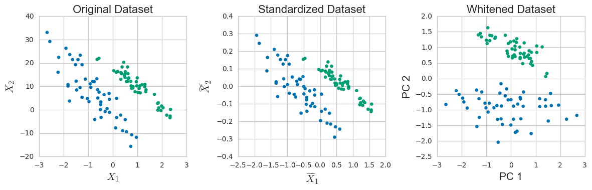
We can extract another useful morsel by thinking about the scaling of $U$. Recall that each singular value corresponds to the length of a semi-axis of an ellipse that describes the column space of $X$. By dividing out the singular value (and multiplying by $\sqrt{n-1}$ to deal with the fact that we started with the covariance) we obtain a transformed dataset which is in some sense spherical:

This process produces a unit variance dataset in a way that can be difficult to achieve by just centering and scaling.

As a final remark, let’s discuss the numerical advantages of using SVD. A basic approach to actually calculating PCA on a computer would be to perform the eigenvalue decomposition of $X^TX$ directly. It turns out that doing so would introduce some potentially serious numerical issues that could be avoided by using SVD.

The problem lies in the fact that on a computer real numbers are represented with finite precision. Since each number is stored in a finite amount of memory there is necessarily a gap between consecutive representable numbers. For double precision floating point numbers, for instance, the relative error between a real number and its closest floating point approximation is on the order of $\varepsilon \approx 10^{-16}$. Algorithms that take this limitation into account are called backward stable. The basic idea is that such an algorithm produces the correct output for an input value that’s within $\varepsilon$ of the value you actually asked about.

If $\tilde \sigma_i$ is the output of a backward stable algorithm calculating singular values for $X$ and $\sigma_i$ is the true singular value, it can be shown that

where $\| X \|$ is a reasonable measure of the size of $X$. On the other hand, a backward stable algorithm that calculates the eigenvalues $l_i$ of $X^TX$ can be shown to satisfy

which when given in terms of the singular values of $X$ becomes

The end result here is that if you are interested in relatively small singular values, e.g. $\sigma_i \ll \| X \|$, working directly with $X$ will produce much more accurate results than working with $X^TX$. Luckily, SVD lets us do exactly that.

Conclusion

There is obviously a lot more to say about SVD and PCA. If you’d like to know more about ways to extend these ideas and adapt them to different scenarios, a few of the references that I have found useful while writing this article are Numerical Linear Algebra by Trefethen and Bau (1997, SIAM) and Principal Component Analysis by Jolliffe (2002, Springer).

If you need a custom data sourcing, transformation and analysis solution, get in touch with us to see how our experts can help you make the most out of your data.